Class Notes

Switching a RMarkdown Article Manuscript from PDF to Word

Sunday, 19 April 2020

This is a quick follow-up to Making RMarkdown the New Way You Write Everything, which among other topics, described how to write your article manuscripts in RMarkdown. The assumption there was that you’d want a nice PDF as output to make sharing your work easy. But what if you need to quickly get a word-formatted version of your article? Now you may be asking yourself, “Why in the name of all that’s good would I ever want that?”

The Problem

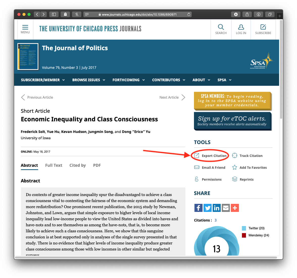
We are in the process of preparing your article for publication. We have noticed that manuscript and the files supplied are in PDF format, and we cannot typeset your article from a PDF file. We would be most grateful if you could re-supply the files for your manuscript within 24 hours by e-mail.

Our preferred format for the manuscript and tables is Word. Optimal resolution for line artwork is 800 dpi and for halftones is 300 dpi. Preferred formats are EPS and TIFF for line artwork, and JPEG for halftones.

Ugh. Right. That’s why.

The Solution

RMarkdown makes converting a manuscript to a .docx fairly easy. The process is not quite seamless, though, so it’s wise I think to duplicate the .Rmd file and rename it with _word. That is, if the paper starts from example_article.Rmd, make a duplicate and call it example_article_word.Rmd.

Step 1. The YAML metadata

Our preferred PDF template, svm-latex-ms2.tex, has all kinds of YAML stuff that the word version will ignore, although it doesn’t actually have to be deleted: fontsize, spacing, citecolor, linkcolor, endnote.1 But author apparently has to be a single string—author: "Frederick Solt, _University of Iowa_"— rather than using name and affiliation, and thanks should be switched to an inline footnote at the end of the title:

title: "An Example Article^[This paper's revision history and the materials needed to reproduce its analyses can be found on Github at <http://github.com/fsolt/example_article>.  Corresponding author: [frederick-solt@uiowa.edu](mailto:frederick-solt@uiowa.edu).]"

The big thing to change, of course, is the output, which should appear as below:

output: 
  word_document:
    reference_docx: word-styles-reference-01.docx
    keep_md: true

The word-styles-reference-01.docx file ensures the references get hanging indents; one could do more here to customize the format, but we don’t care, and even this much probably isn’t really necessary. Anyway, download it here and put it in the same directory with the .Rmd.

Setting keep_md to TRUE has the side effect that the directory of figures is preserved. They’ll all need to be exported as .tiff and .jpeg files, too (let the publisher figure out which format they want to use for each, I think). I’m positive there’s a clever one-liner to do this, and I really want to go look for it, but it took way less than a minute to get the job done in Preview. I’m sure there are equally quick ways to do this in windows. Satisficing, FTW.

Oh, one more thing—my little hack to find the bibliography automatically

bibliography: \dummy{ `r file.path(getwd(), list.files(getwd(), "bib$"))` }

doesn’t seem to mix well with output: word_document. Just call the .bib file directly, e.g., bibliography: "example_article.bib".

Step 2. Figure Captions and Cross-References

The only in-text issue I found is that figure captions don’t have the “Figure X:” prefix and figure cross-references don’t appear. So go into the .Rmd, search for “fig”, and add “Figure 1:”, “Figure 2:” and so on to the figure captions in the code chunks, and add the “1”, “2”, etc., where they go in the text.

Step 3: Bibliography

There are two things to do here. First, add “## References” to the bottom of the .Rmd. Second, carefully look over the output bibliography to catch any differences between how your references are cited in the PDF and how they appear in the word file. (In my case, my .bib includes many unpublished documents that get cited how I want them to in the PDF, but don’t appear right in the .docx; they need to be switched to misc to appear correctly. For each of these items, in my favorite Bib\(\TeX\) software, BibDesk, I needed to cut the Note entry to the clipboard, switch the item to misc, and paste the clipboard into Howpublished.)

So, if any such modifications are necessary, one should create a new, duplicate version of the .bib file with the _word name suffix—remember to change this name in the bibliography: entry of the YAML header of the .Rmd, too—and make the needed changes in that file.

Done!

Not instantaneous, but pretty darn quick, really: a matter of minutes, now that it is all figured out.


  1. I delete it anyway, because I prefer my code clean. You of course can feel free to do you.↩︎

Scraping Data from the Web with rvest

Thursday, 14 March 2019

There are lots of R packages that offer special purpose data-download tools—Eric Persson’s gesis is one of my favorites, and I’m fond of icpsrdata and ropercenter too—but the Swiss Army knife of webscraping is Hadley Wickham’s rvest package. That is to say, if there’s a specialized tool for the online data you’re after, you’re much better off using that tool, but if not, then rvest will help you to get the job done.

In this post, I’ll explain how to do two common webscraping tasks using rvest: scraping tables from the web straight into R and scraping the links to a bunch of files so you can then do a batch download.

Scraping Tables

Scraping data from tables on the web with rvest is a simple, three-step process:

  1. read the html of the webpage with the table using read_html()

  2. extract the table using html_table()

  3. wrangle as needed

As Julia Silge writes, you can just about fit all the code you need into a single tweet!

So let’s suppose we wanted to get the latest population figures for the countries of Latin America from Wikipedia

Step 1: Read the Webpage

We load the tidyverse and rvest packages, then paste the url of the Wikipedia page into read_html()

library(rvest)
## Loading required package: xml2
library(tidyverse)
## ── Attaching packages ──────── tidyverse 1.2.1 ──
## ✔ ggplot2 3.2.1.9000     ✔ purrr   0.3.3     
## ✔ tibble  2.1.3          ✔ dplyr   0.8.3     
## ✔ tidyr   1.0.0          ✔ stringr 1.4.0     
## ✔ readr   1.3.1          ✔ forcats 0.4.0
## ── Conflicts ─────────── tidyverse_conflicts() ──
## ✖ dplyr::filter()         masks stats::filter()
## ✖ readr::guess_encoding() masks rvest::guess_encoding()
## ✖ dplyr::lag()            masks stats::lag()
## ✖ purrr::pluck()          masks rvest::pluck()
webpage <- read_html("http://en.wikipedia.org/wiki/List_of_Latin_American_countries_by_population")

Step 2: Extract the Table

So far, so good. Next, we extract the table using html_table(). Because the last row of the table doesn’t span all of the columns, we need to use the argument fill = TRUE to set the remaining columns to NA. Helpfully, the function will prompt us to do this if we don’t recognize we need to. One wrinkle is that html_table() returns a list of all of the tables on the webpage. In this case, there’s only one table, but we still get back a list of length one. Since what we really want is a dataframe, not a list, we’ll use first() to grab the first element of the list. If we had a longer list and wanted some middle element, we’d use nth(). And we’ll make the dataframe into a tibble for the extra goodness that that format gives us.

latam_pop <- webpage %>% 
    html_table(fill=TRUE) %>%   # generates a list of all tables
    first() %>%                 # gets the first element of the list
    as_tibble()                 # makes the dataframe a tibble
    
latam_pop
## # A tibble: 27 x 10
##    Rank  `Country(or dep… `July 1, 2015pr… `% ofpop.` `Averagerelativ…
##    <chr> <chr>            <chr>                 <dbl>            <dbl>
##  1 1     Brazil           204,519,000           33.1              0.86
##  2 2     Mexico           127,500,000           19.6              1.08
##  3 3     Colombia         48,218,000             7.81             1.16
##  4 4     Argentina        43,132,000             6.99             1.09
##  5 5     Peru             32,721,300             5.05             1.1 
##  6 6     Venezuela        30,620,000             4.96             1.37
##  7 7     Chile            18,006,000             2.92             1.05
##  8 8     Ecuador          16,279,000             2.64             1.57
##  9 9     Guatemala        16,176,000             2.62             2.93
## 10 10    Cuba             11,252,000             1.82             0.25
## # … with 17 more rows, and 5 more variables:
## #   `Averageabsoluteannualgrowth[3]` <chr>,
## #   `Estimateddoublingtime(Years)[4]` <chr>,
## #   `Officialfigure(whereavailable)` <chr>, `Date oflast figure` <chr>,
## #   Source <chr>

Step 3: Wrangle as Needed

Nice, clean, tidy data is rare in the wild, and data scraped from the web is definitely wild. So let’s practice our data-wrangling skills here a bit. The column names of tables are usually not suitable for use as variable names, and our Wikipedia population table is not exceptional in this respect:

names(latam_pop)
##  [1] "Rank"                              "Country(or dependent territory)"  
##  [3] "July 1, 2015projection[1]"         "% ofpop."                         
##  [5] "Averagerelativeannualgrowth(%)[2]" "Averageabsoluteannualgrowth[3]"   
##  [7] "Estimateddoublingtime(Years)[4]"   "Officialfigure(whereavailable)"   
##  [9] "Date oflast figure"                "Source"

These names are problematic because they have embedded spaces and punctuation marks that may cause errors even when the names are wrapped in backticks, which means we need a way of renaming them without even specifying their names the first time, if you see what I mean. One solution is the clean_names() function of the janitor package:1

latam_pop <- latam_pop %>% janitor::clean_names()

names(latam_pop)
##  [1] "rank"                                 
##  [2] "country_or_dependent_territory"       
##  [3] "july_1_2015projection_1"              
##  [4] "percent_ofpop"                        
##  [5] "averagerelativeannualgrowth_percent_2"
##  [6] "averageabsoluteannualgrowth_3"        
##  [7] "estimateddoublingtime_years_4"        
##  [8] "officialfigure_whereavailable"        
##  [9] "date_oflast_figure"                   
## [10] "source"

These names won’t win any awards, but they won’t cause errors, so janitor totally succeeded in cleaning up. It’s a great option for taking care of big messes fast. At the other end of the scale, if you only need to fix just one or a few problematic names, you can use rename()’s new(-ish) assign-by-position ability:

latam_pop <- webpage %>% 
    html_table(fill=TRUE) %>%   # generates a list of all tables
    first() %>%                 # gets the first element of the list
    as_tibble() %>%             # makes the dataframe a tibble
    rename("est_pop_2015" = 3)  # rename the third variable

names(latam_pop)
##  [1] "Rank"                              "Country(or dependent territory)"  
##  [3] "est_pop_2015"                      "% ofpop."                         
##  [5] "Averagerelativeannualgrowth(%)[2]" "Averageabsoluteannualgrowth[3]"   
##  [7] "Estimateddoublingtime(Years)[4]"   "Officialfigure(whereavailable)"   
##  [9] "Date oflast figure"                "Source"

An intermediate option is to assign a complete vector of names (that is, one for every variable):

names(latam_pop) <- c("rank", "country", "est_pop_2015",
                      "percent_latam", "annual_growth_rate",
                      "annual_growth", "doubling_time",
                      "official_pop", "date_pop",
                      "source")

names(latam_pop)
##  [1] "rank"               "country"            "est_pop_2015"      
##  [4] "percent_latam"      "annual_growth_rate" "annual_growth"     
##  [7] "doubling_time"      "official_pop"       "date_pop"          
## [10] "source"

Okay, enough about variable names; we have other problems here. For one thing, several of the country/territory names have their colonial powers in parentheses, and there are also Wikipedia-style footnote numbers in brackets that we don’t want here either:

latam_pop$country[17:27]
##  [1] "El Salvador"               "Costa Rica"               
##  [3] "Panama"                    "Puerto Rico (US)[5]"      
##  [5] "Uruguay"                   "Guadeloupe (France)"      
##  [7] "Martinique (France)"       "French Guiana"            
##  [9] "Saint Martin (France)"     "Saint Barthélemy (France)"
## [11] "Total"

We can use our power tool regex to get rid of that stuff. In the regex pattern below, recall that the double slashes are “escapes”: they mean that we want actual brackets (not a character class) and actual parentheses (not a capture group). Remember too that the .*s stand for “anything, repeated zero or more times”, and the | means “or.” So this str_replace_all() is going to replace matched brackets or parentheses and anything between them with nothing.

And one more quick note on country names: there are lots of variations. If you’re working with data from different sources, you will need to ensure your country names are standardized. Vincent Arel-Bundock’s countrycode package is just what you need for that task. It standardizes names and can convert between names and bunch of different codes as well!

We’ll skip countrycode for now, but while we’re dealing with this variable, we’ll get rid of the observation listing the region’s total population.

latam_pop <- latam_pop %>% 
    mutate(country = str_replace_all(country, "\\[.*\\]|\\(.*\\)", "") %>% 
               str_trim()) %>% 
    filter(!country=="Total")

latam_pop$country[17:nrow(latam_pop)]
##  [1] "El Salvador"      "Costa Rica"       "Panama"           "Puerto Rico"     
##  [5] "Uruguay"          "Guadeloupe"       "Martinique"       "French Guiana"   
##  [9] "Saint Martin"     "Saint Barthélemy"

Another common problem with webscraped tables: are the numbers encoded as strings? Probably so.

latam_pop$official_pop
##  [1] "212,436,000" "122,273,473" "50,767,000"  "43,590,368"  "31,488,625" 
##  [6] "31,028,637"  "18,191,884"  "17,504,400"  "16,176,133"  "11,238,317" 
## [11] "10,911,819"  "10,985,059"  "10,075,045"  "8,576,500"   "6,854,536"  
## [16] "6,071,045"   "6,520,675"   "4,832,234"   "3,764,166"   "3,548,397"  
## [21] "3,480,222"   "403,314"     "388,364"     "239,648"     "35,742"     
## [26] "9,131"
str(latam_pop$official_pop)
##  chr [1:26] "212,436,000" "122,273,473" "50,767,000" "43,590,368" ...

Yep. So let’s replace the commas with nothing and use as.numeric() to make the result actually numeric.

latam_pop <- latam_pop %>% 
    mutate(official_pop = str_replace_all(official_pop, ",", "") %>%
               as.numeric())

latam_pop$official_pop
##  [1] 212436000 122273473  50767000  43590368  31488625  31028637  18191884
##  [8]  17504400  16176133  11238317  10911819  10985059  10075045   8576500
## [15]   6854536   6071045   6520675   4832234   3764166   3548397   3480222
## [22]    403314    388364    239648     35742      9131
str(latam_pop$official_pop)
##  num [1:26] 2.12e+08 1.22e+08 5.08e+07 4.36e+07 3.15e+07 ...

One last issue is to get the dates for these population figures into POSIXct format. This is complicated a bit by the fact for some countries we only have a year rather than a full date:

latam_pop$date_pop
##  [1] "April 19, 2020"    "July 1, 2016"      "April 19, 2020"   
##  [4] "July 1, 2016"      "June 30, 2016"     "2016"             
##  [7] "2016"              "April 19, 2020"    "July 1, 2015"     
## [10] "December 31, 2014" "2015"              "2016"             
## [13] "2016"              "July 1, 2015"      "2016"             
## [16] "June 30, 2012"     "2016"              "June 30, 2015"    
## [19] "July 1, 2015"      "July 1, 2014"      "June 30, 2016"    
## [22] "January 1, 2012"   "January 1, 2012"   "January 1, 2012"  
## [25] "January 1, 2012"   "January 1, 2012"

We deal with this using if_else() and str_detect() to find which dates begin (^) with a digit (\\d), and then let the lubridate package’s parse_date_time() function know that those are years and the rest are in “month day, year” format.

latam_pop <- latam_pop %>% 
    mutate(date_pop = if_else(str_detect(date_pop, "^\\d"),
                              lubridate::parse_date_time(date_pop,
                                                         "y"),
                              lubridate::parse_date_time(date_pop,
                                                         "m d, y")))

latam_pop$date_pop
##  [1] "2020-04-19 UTC" "2016-07-01 UTC" "2020-04-19 UTC" "2016-07-01 UTC"
##  [5] "2016-06-30 UTC" "2016-01-01 UTC" "2016-01-01 UTC" "2020-04-19 UTC"
##  [9] "2015-07-01 UTC" "2014-12-31 UTC" "2015-01-01 UTC" "2016-01-01 UTC"
## [13] "2016-01-01 UTC" "2015-07-01 UTC" "2016-01-01 UTC" "2012-06-30 UTC"
## [17] "2016-01-01 UTC" "2015-06-30 UTC" "2015-07-01 UTC" "2014-07-01 UTC"
## [21] "2016-06-30 UTC" "2012-01-01 UTC" "2012-01-01 UTC" "2012-01-01 UTC"
## [25] "2012-01-01 UTC" "2012-01-01 UTC"

And we’re done! One point worth considering is whether you want this particular scrape to be reproducible. Sometime you won’t—maybe the page you’re scraping is updated regularly, and you always want the latest data. But if you do want to be sure to be able to reproduce what you’ve done in the future, I recommend you take a second, go to the Internet Archive, archive the page, and then scrape the archived page instead of the live one.

Scraping Files

It’s also pretty common to want to get a bunch of files linked from a website. Consider this example from my own work on the Standardized World Income Inequality Database. The SWIID depends on source data on income inequality from international organizations and national statistical offices around the world, including Armenia’s Statistical Committee (ArmStat). ArmStat has a annual report on food security and poverty that includes a chapter titled “Accessibility of Food” that has some data on income and consumption inequality that I want.

Here’s the page with the list of poverty reports:

Clicking on the top link shows a list of chapters. Note the chapter on “Accessibility of Food”:

Clicking on that pdf icon shows the pdf file of the chapter, where we can see, if we scroll down a bit, the table with the lovely data:

But again, we want to download that file for that chapter for every one of the annual reports listed on that first page. We could go carefully down the list of all the reports, pick out the annual reports, click through the chapters over and over, but there’s more than a dozen annual reports here, and we’re still at the start of the alphabet as far as countries go. Further, there’ll be another new annual report next year. We need to have this process automated.

Thinking about it a moment, this is maybe a particularly tricky scraping job because we need to:

  1. use rvest to get the links for the reports we want from the main page on poverty, and then

  2. follow each of those links to get the link for the chapter we want, and, after we have all those links, then

  3. we can download all the chapter files and extract the data we want from them. (Reading pdfs into R is another great data acquisition skill, but I think it merits a post of its own, so for now we’ll stop once we have all the files we want.)

In a more straightforward scraping job, step 2 wouldn’t be necessary at all, but this sort of arrangement isn’t all that uncommon (think of articles in issues of journals, for another example), and it will give us a chance to practice some of our data wrangling skills.

And in the very most straightforward cases, as Raman Singh Chhína reminded me here, the links to files we want will fit some consistent pattern, and even step 1 won’t be necessary as we can simply construct the list of links we need along the lines of: needed_links <- str_c("https://suchandsuch.org/files/annualreport", 2006:2018, ".pdf"). Then we can skip straight to step 3.

But let’s roll up our sleeves and take on this harder job.

Step 3: Getting! All! the! Files!

This is actually straightforward, now that we have a tibble of report titles and links to chapter files. The download.file() function will save the contents of a link (its first argument) to a filepath (its second argument) and the walk2() function allows you to pass a pair of vectors to a function to iteratively use as its two arguments (first the first element of each vector, then the second element of each vector, and so on). We’ll use str_extract() to get the year of the report from its title, and use it to make a file name for the pdf with str_c(). But first we should create a directory to save those files in. And after each download, we’ll insert a brief pause with Sys.sleep(3) to be sure that were not hammering the server too hard. Maybe not really necessary this time, given that we’re getting just 14 files, but it’s the considerate thing to do and a good habit.

dir.create("armstat_files")

walk2(reports_links$report_title, reports_links$chapter_link,
      function(report_title, chapter_link) {
    pdf_path <- file.path("armstat_files",
                          str_c("armstat", 
                                str_extract(report_title, "\\d{4}"),
                                ".pdf"))
    download.file(chapter_link, pdf_path)
    Sys.sleep(3)
})

And that’s that. And remember, use your new powers for good, not for evil. Be sure to respect the terms of service of any website you might want to scrape.


  1. Remember, if you haven’t installed it before, you will need to download janitor to your machine with install.packages("janitor") before this code will work.↩︎

Getting an Academic Website Online with blogdown

Tuesday, 29 January 2019

Okay, you’ve gotten RStudio installed and linked up with GitHub. You’ve gotten started with RMarkdown, and you’re ready to use it to write all of your academic documents so your work will be reproducible. The next step is to get an academic website to display your work—even your early, early work—online. Conveniently, we can use RStudio, GitHub, and RMarkdown to do that, too!

Before we start, you might be asking yourself why you’d want to get your work online. David Robinson, Chief Data Scientist at DataCamp has done the best job I’ve seen articulating the answer to just this question. In short, he argues that putting your work online gives you practice communicating your research (blog posts are a great way to get that difficult first draft written); provides a way to get quick feedback; and attracts an audience to your work that can include future collaborators and even employers. Most importantly, it lets you teach people at a scale you’re not likely to reach any other way. Anyway, you should read his whole post on the value of blogging your work with data.1 You really do want to do this.

Building Your Own Website in Ten Easy Steps

Ten steps seems like a lot, but they’re seriously easy.

  1. We start by creating a new project repo on GitHub and opening it in RStudio (you remember how to do that, right?). Call it whatever you like; the name won’t be important, as long as you remember it.

  2. The R package we need for this task is called blogdown, which is built on top of a framework for building websites called Hugo. Install them both by typing this into the console, in the bottom left pane of RStudio:

    install.packages("blogdown")    # install the blogdown package
    blogdown::install_hugo()        # install Hugo (a function in the blogdown package)
  3. In the lower right pane of RStudio, you’ll see the Files tab; as advertised, it provides an alternate way of browsing through your files. The first file listed in your new repo should be called .gitignore. More truth in advertising: this file is where you list documents for this project that you don’t want to save in the project’s git (and, in turn, GitHub) repo. Open it up and paste in the following:

    .Rproj.user
    .Rhistory
    .RData
    .Ruserdata
    .DS_Store
    Thumbs.db
    blogdown/
    public/

    The first four lines were already there, the fifth and sixth are irrelevant system files on Macs and Windows machines respectively, and the last two are directories (that is, folders) that blogdown uses that we don’t need backed up.

  4. Now we’re ready to build the site. There are a ton of different Hugo themes, but as I’ve mentioned before, I’m super-fussy, so I made my own, which we’ll be using here. Let’s get started:

    blogdown::new_site(theme = "fsolt/hugo-prof", theme_example = TRUE)

    Building the site also automatically starts serving it locally–a tiny rendition of our site pops up in the lower left pane of RStudio, in the Viewer tab. Later, you can start serving the site by clicking on RStudio’s Addins button (right at the top of the window, under the title bar) and selecting “Serve Site.” Anyway, back in the Viewer tab, at the top left, go ahead and click on the little square with an arrow to “Show in a new window.” It’ll pop up in your browser, and it should look, ah, vaguely familiar. Anyway, new_site also created a bunch of files, so we should commit them to git and push the changes to GitHub. Go to the Git tab in the upper right pane of RStudio, click on the “Staged” checkboxes next to each file, and hit the “Commit” button. In the upper right of the review-changes window that pops up, type a message that tells what this commit ‘will’ do compared to the previous commit: “add hugo-prof theme” does the trick here. The idea is to provide enough information so that you will later be able to scroll back through the commit history and identify the point in time you’re looking for. Then hit the “Commit” button to save your changes to your repo on your machine. Close the pop-up, and then hit the up-arrow button that says “Push.” That sends your changes to your repo on GitHub. (Sorry, you knew all this already. Ah, well, repetition does help sometimes, I think.)

    This approach, otoh, will probably make “future-you” say things about “current-you” that are really mean.

  5. Hugo allows you to customize themes using the config.toml file. So click the Files tab (again, that’s in the lower left pane), open the config.toml file, and let’s get your page set up better for your needs. Here’s what that file holds:

    baseurl = "http://example.netlify.io/"
    relativeurls = false
    languageCode = "en-us"
    title = "Your Name"
    theme = "hugo-prof"
    googleAnalytics = ""
    disqusShortname = ""
    ignoreFiles = ["\\.Rmd$", "_files$", "_cache$"]
    uglyURLS = false
    enableEmoji = true
    blogdir = "blog"
    
    [permalinks]
        post = "blog/:year/:month/:day/:slug/"
    
    [[menu.main]]
        name = "Home"
        url = "/"
        weight = 1
    [[menu.main]]           # comment out this row, plus the name, url, and weight to omit  
       name = "Research"    
       url = "/research/"
       weight = 2
    [[menu.main]]           # comment out this row, plus the name, url, and weight to omit 
       name = "Teaching"
       url = "/teaching/"
       weight = 3
    [[menu.main]]           # comment out this row, plus the name, url, and weight to omit 
        name = "Blog"
        url = "/blog/"
        weight = 4
    [[menu.main]]
        name = "CV"
        url = "/cv.pdf"
        weight = 5
    
    [params]
        description = "Your name and a few keywords on your academic interests" 
        subtitle = "A few keywords on your academic interests"
        home_text = "A paragraph or so of professional bio.  Write it in the config.toml file---it's called home_text---as one long string."
    
        author = "Your Name"
        dateFormat = "2006/01/02"
        email = "your_email@uppermidwest.edu"
        github_username = "your_github_username"
        twitter_username = "your_twitter_username"  # leave empty quotes to omit
        gscholar_code = "your_gscholar_code"        # leave empty quotes to omit    
    
        page_color = "white"
        text_color = "black"
        link_color = "rgb(0, 0, 152)"
        hover_color = "rgb(255, 102, 0)"
    
    
        # options for highlight.js (version, additional languages, and theme)
        highlightjsVersion = "9.12.0"
        highlightjsCDN = "//cdnjs.cloudflare.com/ajax/libs"
        highlightjsLang = ["r", "yaml"]
        highlightjsTheme = "github"
    
        MathJaxCDN = "//cdnjs.cloudflare.com/ajax/libs"
        MathJaxVersion = "2.7.5"

    Right off, you’ll want to change the title of the site (line 4); the description, subtitle, and home_text (lines 38-40); plus the author, email, github_username, twitter_username, and gscholar_code (lines 42-47). As the comments in the file tell you, if you don’t yet have the twitter (if not, I really think you should give it a try) or a Google Scholar account (it’s probably too soon for you to have one of those, otoh), you can leave the quotes empty and the link for them will disappear. After you’ve made the appropriate changes, save the file. Check out the site in your browser—it should show your changes. Save, commit (“add personal info” is a fine message), and push.

  6. There’s a lot more you can do to customize your site in the config.toml file. See the five [[menu.main]] items? They are at lines 16-35 of the file. They specify the links that will appear in the sidebar to navigate your site. You can use hashtags to ‘comment them out,’ that is, to make them appear to be comments for humans rather than actual code. While we’re here, let’s comment out the teaching and research links to make them disappear. Of course, when you are further along in the program and have more to share on these fronts, delete the #s and bring them back. And then if you’d like to add another item to the sidebar, maybe a dedicated page for your dissertation or some other big project, you can do that easily: just add four lines for it, starting with [[menu.main]] and including a name (what you want the link to say), url (where you want the link to go), and weight (where in the list you want the link to appear). Save, commit (“revise sidebar”), and push.

  7. My color preferences are, um, maybe somewhat idiosyncratic, and you doubtless have your own in any event. You can change the colors of the page here, too, using the page_color, text_color, link_color, and hover_color parameters (lines 49-52 in the file). These parameters accept any color that HTML does, so you can specify a name, a hex code, an rgb value, whatever. Plugging in the following, for example, will give your page a Hawkeye makeover:

        page_color = "#f0f0f0"
        text_color = "#424242"
        link_color = "black"
        hover_color = "#fcd116"

    Save to preview the results in your browser, commit (“change to Hawkeye color scheme”), and push.

  8. Time for content. Intuitively enough, Hugo puts that in the content/ directory. Remember the CV you learned to make for yourself last week in RMarkdown? Right now, your site is showing the one Steven V. Miller made for William Sealy Gosset. Since you’re a student, not the Student, you’ll want to change that right away. This is a two-step process: (1) put your CV file, “SoltCV.pdf” for example,2 in the content/ directory, and (2) change the url under the [[menu.main]] item for the CV in the config.toml file at line 34 from "/cv.pdf" to the name of your CV file, keeping the slash (and the quotes). Commit (“replace CV”) and push.

  9. David Robinson’s got you all fired up and ready to blog about your data? Good! Click the “Addins” button again (remember, it’s just under the title bar) and select “New Post.” A pop-up will appear with blanks for the title of the post and so on. Be sure to choose the RMarkdown format so you can include R code and output. The hugo-prof theme will put your post at the top of the blog page, with older posts appearing reverse chronologically below. Each post also has its own dedicated page, linked from the main blog page via the post’s title. As you work on the post, save regularly, commit, and push. Each time you save, the locally served version of your website will update in your browser so that you can see exactly how your page is going to look.

  10. When you’re ready to have separate pages for your research and teaching, first remember to uncomment the relevant lines in the config.toml file that we commented out above. Then, you’ll need to edit the file content/teaching/_index.Rmd to add your teaching interests, experience, and courses taught and content/research/_index.Rmd to add your research interests, projects, conference presentations, working papers, and publications.

And we’re done!

Publishing Your Website Using Netlify

Once you have your website looking good on your own machine, you’re ready to get it online. Go to Netlify, which has a good free tier, and hit the button to sign up for an account. Choose to sign up with your GitHub account.

After you click through the sign up process, hit the button that says “New site from Git.” On the next page, under the “Continuous Deployment” header, hit the GitHub button.

Then, after an authorization from GitHub that should just pop up and dismiss itself, you’ll get to choose the repo you want to publish. That would be the one with the name you chose in the very first step of building your site . . . I told you to remember that name!3

Finally, you have to specify the build settings. For the build command, enter “hugo”. For the publish directory, enter “public”. The branch to deploy is “master”. Hit the button to deploy the site, and that’s it. Your site is online!

Changing the Domain Name

By default, Netlify will provide your website with some random address (for cmcr-class, I got boring-mayer-5d40c1.netlify.com). There are a number of ways to get a more presentable address. The quickest and easiest way is to simply rename the site on Netlify: if you’re not still there, log into Netlify and choose your site, then click on Settings. Under “Site details,” you’ll see “Site information” (the first bit of which will be the “Site name,” which in turn should still display that random address Netlify assigned you). At the bottom of “Site details” is a button labelled “Change site name.” Clicking there will let you choose a different subdomain, that is, all the stuff before .netlify.com. As long as no one’s beat you to it, you can have pretty much any name you want, so definitely do this.

screenshot of renaming the cmcr-class site on Netlify

Your next step up in customization—requiring only a bit more effort and no more expense—is to get a free rbind.io subdomain from RStudio. Submit the request form (cleverly disguised as a GitHub issue) and wait for one of the extremely good-hearted volunteers who provide this service to get back to you. For me, this only took about an hour, if that even, but if it takes longer, please be patient. Follow the directions in their response (#1) to reconfigure Netlify to use your new custom rbind domain. When you do this, Netlify will warn you that rbind.io is owned by someone else or some such. Don’t panic. You knew that already; you’re not stealing it. Just click through. It’ll be fine.

screenshot of rbind.io response

Yep, I got the “Check DNS configuration” hint from Netlify after adding the rbind subdomain (#2). And, yep, I ignored it. Easy. Here’s the tl;dr on #3: create a plain text document in the project directory for your website called _redirects with the following contents:

http://cmcr-class.rbind.io/*    https://cmcr-class.rbind.io/:splat  301!
https://cmcr-class.netlify.com/*  https://cmcr-class.rbind.io/:splat  301!

Be sure to swap out cmcr-class for whatever you named your subdomain, of course. The first line redirects any nonsecure HTTP links to your site to secure HTTPS links. The second ensures that anyone who happens to try to visit your site via netlify.io gets redirected to your preferred rbind.io address so that all of your visitors will have the same address for any given page. And then you’re done.

The last choice, if an rbind.io subdomain isn’t custom enough for you, if you just need the ultimate in domain name customization, you can (wait for it) buy a custom domain name. Custom domains are generally pretty cheap, up to maybe $10 a year, and they require a bit more configuring, but don’t let that scare you off: as long as you choose your domain reasonably carefully, you’re only going to have to do this work once. Directions from Netlify are here, and the company you buy the domain from will likely have directions for you too.

Whatever level of customization you choose, go back now to your config.toml file and on the first line, put your new address in as the baseurl.

You can add other bells and whistles, like Google Analytics or Disqus comments, pretty easily with blogdown, too. To explore all the details of the package, see Xie, Yihui, Amber Thomas, and Alison Presmanes Hill. 2017. blogdown: Creating Websites with R Markdown. CRC Press. Having a website is an important way of sharing your work, every academic should have one, and with blogdown it’s easy to set up and maintain your own. Let me know when your site is up!


  1. David also just gave a keynote talk at rstudio::conf 2019 titled “The Unreasonable Effectiveness of Public Work” (slides , video) worth checking out, too.↩︎

  2. I really recommend you include your name in the filename, rather than just calling the file cv.pdf like Gosset’s. On the off chance someone excitedly downloads your CV to show to their colleagues as just the sort of person who should be hired, you don’t want to force them to pause and rename the file before forwarding it to the hiring committee. The moment might quickly pass, after all. If that hypothetical is too outlandish, you should instead view it as a specific case of the general rule that file names should convey useful information.↩︎

  3. Of course, you could just read it off of the title bar of your RStudio window.↩︎

Making RMarkdown the New Way You Write Everything

Tuesday, 22 January 2019

RMarkdown is just super-great. To start, it’s plain text, so in a pinch you can read or edit it with basically anything. Next, its formatting is, at least for the most part, easy to remember and easy to interpret. And because it’s RMarkdown, it lets you mix text and R code so that all of your work is in the same document, making it easy for others (and your future self) to see exactly what you did and, if desired, reproduce your work. Finally, it’s incredibly versatile, so you can use it for all your writing.

Here, I’m going to talk about how to get yourself set up to write three important kinds of academic documents in RMarkdown: articles (and the like, including seminar papers), syllabi, and CVs.

Since all of these are documents we will want as PDFs (as opposed to web pages), you’ll need to install \(\LaTeX\) on your computer. The easiest way to do this is by using the tinytex package:

install.packages("tinytex")
tinytex::install_tinytex()

If you have a Mac, you will also need to install XQuartz before continuing.

Okay, let’s get started!

Articles

Start any research project you have with a fresh new project repo–create it on GitHub and open it in RStudio (you remember how to do that, right?).1 Then go to the Files tab in the lower right pane of RStudio, click on New Folder button, and call the new folder “paper” (we’ll worry about other directories that you might need in a project repo another time).

In this directory, we’re going to put three separate files to produce the pretty PDF output we want: the RMarkdown file, which is where you write up your research; a Bib\(\TeX\) file, which contains bibliographic information about the sources you cite; and a template file, which specifies how the final output should look. There’s an example repo here. I’m going to discuss the three files in reverse order, from the one that requires the least attention from you to the one that needs the most.

The Template

There are many article templates out there; there’s even an R package called rticles that makes starting a new draft extra easy. The journals that package’s templates are modelled on lean toward the physical sciences, though, so instead we’re going to work with a template originally written by our fellow political scientist Steven V. Miller and slightly modified by me.2 Anyway, the file is called svm-latex-ms2.tex; put a copy of it in your paper directory each time you start an article project. If you find a different template you’d like to use, just put that in there instead. And that’s that.

The Bib\(\TeX\) File

If we want RMarkdown to automatically generate our bibliography (and we darn sure do), we need to provide information on all of the sources we’re citing. That’s what the Bib\(\TeX\), or .bib, file is for. Whenever you come across an article that you know you’re going to need later, or think you might need later, or just find interesting, you add it to your personal Bib\(\TeX\) file. So how exactly do you do that?

Unless you’re a dedicated Zotero user, your first step will be to get some Bib\(\TeX\) reference manager software.3 If you’re a Mac user like me, give BibDesk a try; I’ve been using it for many, many years. If not, JabRef is the standard. Then, as you’re doing your reading, keep your personal Bib\(\TeX\) file open in that reference manager. You’ll see that pretty much all journals have a button labelled “export citation” or some such. Hit the button, choose BibTeX format, and click through. Depending on the journal publisher, this may download a small .bib file or pop open a new window. If the former, drag the downloaded file your personal Bib\(\TeX\) file in your reference manager to add the new source; if the latter, copy the text, click on your personal Bib\(\TeX\) file, and then paste. This should add the new source. Then—and this is important for friction-free writing later—take a minute and double-check all the entries in the reference manager. Some journals’ citation exports only include first initials, not the whole first name. Make sure the cite key (more on cite keys below) matches whatever convention you choose to adopt. And so on. If you’re careful right when you add a source, you’ll never have to worry about any errors in your bibliographies ever again.

Keep all your sources in your personal Bib\(\TeX\) file: it’ll get long, but since it’s just plain text, never really big. Make sure it gets backed up!4 But each project repo should have its own Bib\(\TeX\) file as well. That way, your project repo is self-contained—it doesn’t rely on files that are located elsewhere on your computer. Just make a new Bib\(\TeX\) file for each project, keep it in the paper directory, and drag sources to it from your personal Bib\(\TeX\) file as you cite them. Just be sure that you only add new sources to your personal Bib\(\TeX\) file and not directly to any project’s file, so that you always know all the sources you’ve entered are in one place and you never end up duplicating that work.

The RMarkdown File

The RMarkdown file is where you’re going to put nearly all of your attention as you’re writing: it contains all of your text and R code. The trick to using RMarkdown to write a beautifully formatted article is in the front matter, which is called the YAML header. (YAML stands for Yet Another Markup Language. Those kidders.) Anyway, let’s look at the header in the example_article.Rmd file:

---
output: 
  pdf_document:
    citation_package: natbib
    keep_tex: false
    fig_caption: true
    latex_engine: pdflatex
    template: svm-latex-ms2.tex
title: "An Example Article"
thanks: "The paper's revision history and the materials needed to reproduce its analyses can be found [on Github here](http://github.com/fsolt/example_article). Corresponding author: [frederick-solt@uiowa.edu](mailto:frederick-solt@uiowa.edu). Current version:  `r format(Sys.time(), '%B %d, %Y')` ."
author:
- name: Frederick Solt
  affiliation: University of Iowa
abstract: "Here's where you write 100 to 250 words, depending on the journal, that describe your objective, methods, results, and conclusion."
keywords: "these, always seem silly, to me, given google, but regardless"
date: " `r format(Sys.time(), '%B %d, %Y')` "
fontsize: 11pt
spacing: single
bibliography: \dummy{ `r file.path(getwd(), list.files(getwd(), "bib$"))` }
biblio-style: apsr
citecolor: black
linkcolor: black
endnote: no
---

The stuff you’ll want to change here is pretty obvious, I think. For now at least, definitely leave everything under output: alone; there’s no need to change anything with R code either, except maybe if you would want to freeze the date for some reason. For more detail on each entry in the YAML header, see Steven V. Miller’s post on his template.

The example file also includes examples of pretty much everything you’re likely to want to do in an article manuscript: headings, footnotes, embedded R code (and how to hide it), plots with captions and how to refer to them, block quotes, comments (that is, notes to self), and, of course, citations.

Addendum: One more thing we need to get our bibliographies formatted in APSR style is (drumroll) the APSR bibliography style file. Download it from here (right-click to get a contextual menu, then select “Download Linked File” or “Save Target As…” or whatever similar option your browser gives you). Now we have to (1) put this file somewhere safe, and (2) let R know where it is. For (1), on a Mac, go to the Finder, then use the Go menu, select Go to Folder…, and enter Users/your_own_username/Library/ (this folder is hidden by default). Make a folder called texmf there, make one. On Windows, make a texmf folder within your user at C:\Users\your_own_username. Inside the texmf folder, make a bibtex folder. Inside that, make a bst folder.5 Drop the apsr.bst file there. Okay, on to (2). First, install the usethis package: install.packages("usethis"). Then past this usethis::edit_r_environ() into the console to open the .Renviron file, which is ordinarily hidden. Add the following line to that file but make sure to replace the example (Mac) path below with the path to the bst folder you just made, save, and restart R from RStudio’s Session menu.

BSTINPUTS="/Users/your_own_username/Library/texmf/bibtex/bst"

Troubleshooting: \(\LaTeX\), unfortunately, doesn’t play nice with filepaths with spaces in them—that is, if there are any spaces in the names of any of the folders your .Rmd file is nested in, and it looks for a separate .bib file (at least the way I have coded it up in this template), RStudio’s knit button won’t be able to make you a pretty PDF. Correct this as you see fit. Personally, my filepaths tend to look like this: Users/fsolt/Projects/whatever_title/paper/whatever_title.Rmd.

All right, now we’re ready to rock this.

Syllabi

To write a syllabus in RMarkdown, you’ll need to start with a good template. Fortunately, Steven V. Miller has made one for this purpose too: svm-latex-syllabus.tex. And, of course, you’ll need an RMarkdown file with the appropriate YAML header. Steve describes the details in his blog post on the template, so I’ll skip that here. He also writes in that post about how to automatically generate the dates you need for your course schedule, but nowadays there’s an easier way of doing that I want to show you. Put this chunk near the top of your document:

```{r include = FALSE}
library(tidyverse)
library(lubridate)

firstday <- "2019-01-15"
    
meetings <- ymd(firstday) + c(0:15) * weeks(1)

meeting_headers <- paste0("Week ", 1:16, ", ", months(meetings), " ", day(meetings))

```

Then you can make headers for each week with

##  `r meeting_headers[1]` : Something Interesting

which will display as

Week 1, January 15: Something Interesting

Neat, huh? The next time you teach, instead of fussing with all the dates, you just have to change firstday in the chunk above to the first day your class meets in the new semester, and that’s it. More time to update the readings!

Speaking of readings, sadly, I don’t think there’s a good Bib\(\TeX\) integration option for RMarkdown syllabi yet. Being extremely picky, I want something that formats full mid-document bibliographic citations, in complete APSR format, with links to the reading online. I suppose I should dig more on this, but in the meantime I’m just typing them in 😢. You’ll find an example repo here and the RMarkdown syllabus for this very course is here.

CV

Finally, let’s do your CV, too. Our RMarkdown template hero, Steven V. Miller, has us covered there as well. The template is here and his post describing how to put it to use is here. And for once, at least, I don’t have much to add.

So there you go: articles, syllabi, and CVs are easy and beautiful in RMarkdown. Now you can write up not just your research reproducibly, but your teaching and professional documents as well.


  1. There’s really no reason not to have a separate project repo for every project: you have unlimited free repos on GitHub, and the marginal space used on your drive is truly tiny. The main advantage is that having a project repo for each project keeps your work organized. I keep all of my project repos together in a directory called “projects” in my Documents folder.↩︎

  2. There are a couple of little changes that are in there just because I’m hopelessly fussy, but one important one that allows us to easily keep our Bib\(\TeX\) file right in the project repo. To Steve, in addition to my thanks for your great work on this, I owe you a PR. To everyone else, just like everything else having to do with templates, you don’t have to worry about it.↩︎

  3. A Bib\(\TeX\) file is just more plain text, so you can write or edit it in just about anything, but dedicated software makes it much nicer to work with.↩︎

  4. If you don’t have another backup solution already in place for your work, start a GitHub repo for it! This isn’t ideal, really, because it requires you to take an extra, conscious step going of opening that repo in RStudio and backing it up. Unlike your other work, you’re not already in the relevant RStudio project to edit the file, so you don’t get the visual prompt in RStudio’s git pane (in the upper right) that the file has been modified and needs to be committed and pushed. So some other backup solution (Time Machine, Resilio Sync, a cloud backup provider, or something else that’s automatic) is really, really preferable.↩︎

  5. There’s a chance that you’ll find at least some of these folders in these locations already. If so, just use the ones you’ve got; don’t make more.↩︎