There are lots of R packages that offer special purpose data-download tools—Eric Persson’s gesis is one of my favorites, and I’m fond of icpsrdata and ropercenter too—but the Swiss Army knife of webscraping is Hadley Wickham’s rvest package. That is to say, if there’s a specialized tool for the online data you’re after, you’re much better off using that tool, but if not, then rvest will help you to get the job done.
In this post, I’ll explain how to do two common webscraping tasks using rvest: scraping tables from the web straight into R and scraping the links to a bunch of files so you can then do a batch download.
Scraping Tables
Scraping data from tables on the web with rvest is a simple, three-step process:
read the html of the webpage with the table using
read_html()extract the table using
html_table()wrangle as needed
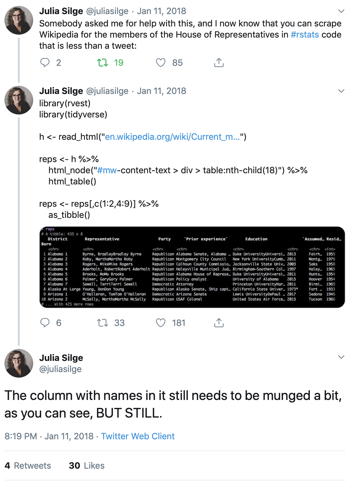
As Julia Silge writes, you can just about fit all the code you need into a single tweet!
So let’s suppose we wanted to get the latest population figures for the countries of Latin America from Wikipedia
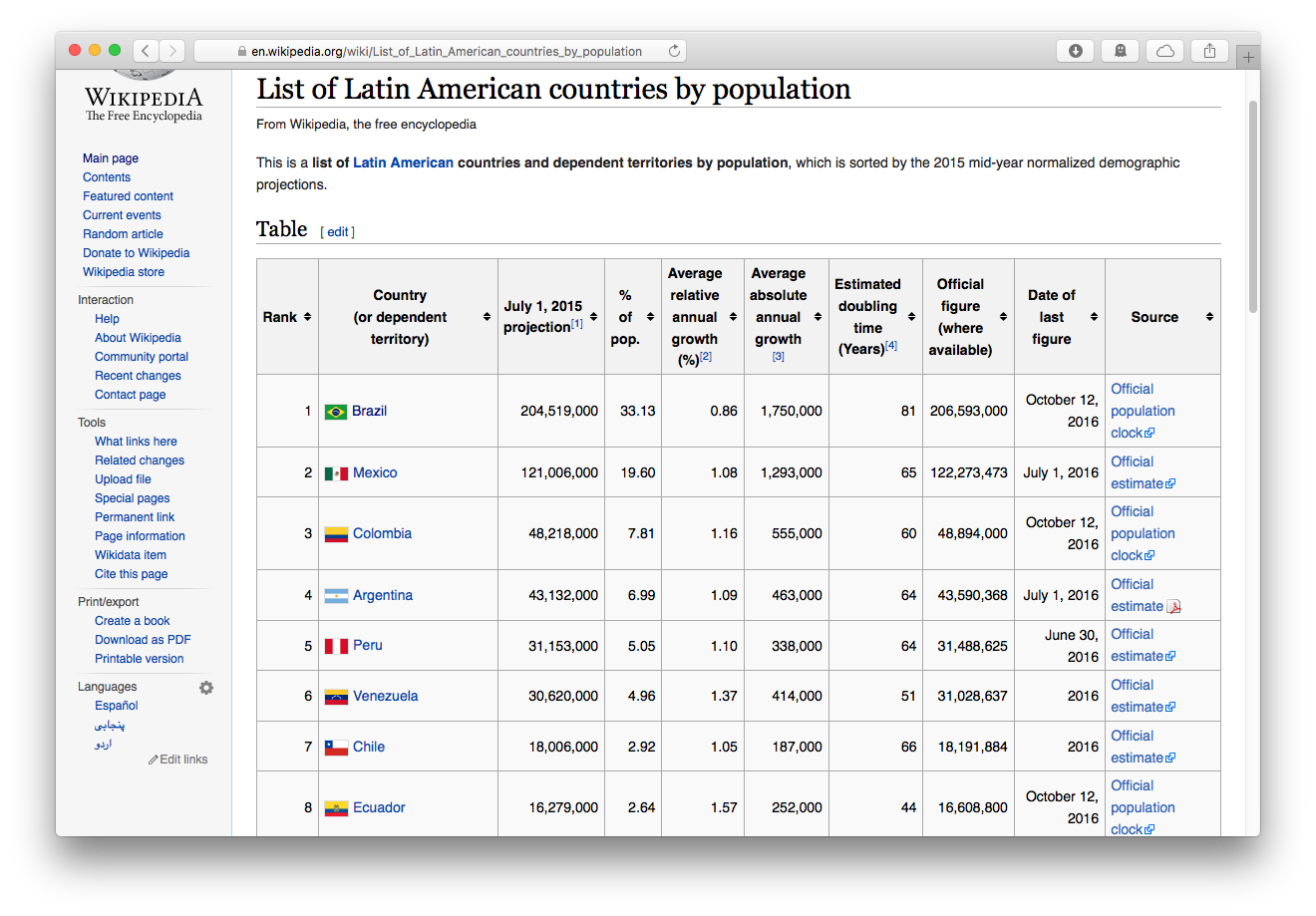
Step 1: Read the Webpage
We load the tidyverse and rvest packages, then paste the url of the Wikipedia page into read_html()
library(rvest)## Loading required package: xml2library(tidyverse)## ── Attaching packages ──────── tidyverse 1.2.1 ──## ✔ ggplot2 3.2.1.9000 ✔ purrr 0.3.3
## ✔ tibble 2.1.3 ✔ dplyr 0.8.3
## ✔ tidyr 1.0.0 ✔ stringr 1.4.0
## ✔ readr 1.3.1 ✔ forcats 0.4.0## ── Conflicts ─────────── tidyverse_conflicts() ──
## ✖ dplyr::filter() masks stats::filter()
## ✖ readr::guess_encoding() masks rvest::guess_encoding()
## ✖ dplyr::lag() masks stats::lag()
## ✖ purrr::pluck() masks rvest::pluck()webpage <- read_html("http://en.wikipedia.org/wiki/List_of_Latin_American_countries_by_population")Step 2: Extract the Table
So far, so good. Next, we extract the table using html_table(). Because the last row of the table doesn’t span all of the columns, we need to use the argument fill = TRUE to set the remaining columns to NA. Helpfully, the function will prompt us to do this if we don’t recognize we need to. One wrinkle is that html_table() returns a list of all of the tables on the webpage. In this case, there’s only one table, but we still get back a list of length one. Since what we really want is a dataframe, not a list, we’ll use first() to grab the first element of the list. If we had a longer list and wanted some middle element, we’d use nth(). And we’ll make the dataframe into a tibble for the extra goodness that that format gives us.
latam_pop <- webpage %>%
    html_table(fill=TRUE) %>%   # generates a list of all tables
    first() %>%                 # gets the first element of the list
    as_tibble()                 # makes the dataframe a tibble

latam_pop
## # A tibble: 27 x 10
## Rank `Country(or dep… `July 1, 2015pr… `% ofpop.` `Averagerelativ…
## <chr> <chr> <chr> <dbl> <dbl>
## 1 1 Brazil 204,519,000 33.1 0.86
## 2 2 Mexico 127,500,000 19.6 1.08
## 3 3 Colombia 48,218,000 7.81 1.16
## 4 4 Argentina 43,132,000 6.99 1.09
## 5 5 Peru 32,721,300 5.05 1.1
## 6 6 Venezuela 30,620,000 4.96 1.37
## 7 7 Chile 18,006,000 2.92 1.05
## 8 8 Ecuador 16,279,000 2.64 1.57
## 9 9 Guatemala 16,176,000 2.62 2.93
## 10 10 Cuba 11,252,000 1.82 0.25
## # … with 17 more rows, and 5 more variables:
## # `Averageabsoluteannualgrowth[3]` <chr>,
## # `Estimateddoublingtime(Years)[4]` <chr>,
## # `Officialfigure(whereavailable)` <chr>, `Date oflast figure` <chr>,
## # Source <chr>Step 3: Wrangle as Needed
Nice, clean, tidy data is rare in the wild, and data scraped from the web is definitely wild. So let’s practice our data-wrangling skills here a bit. The column names of tables are usually not suitable for use as variable names, and our Wikipedia population table is not exceptional in this respect:
names(latam_pop)## [1] "Rank" "Country(or dependent territory)"
## [3] "July 1, 2015projection[1]" "% ofpop."
## [5] "Averagerelativeannualgrowth(%)[2]" "Averageabsoluteannualgrowth[3]"
## [7] "Estimateddoublingtime(Years)[4]" "Officialfigure(whereavailable)"
## [9] "Date oflast figure" "Source"These names are problematic because they have embedded spaces and punctuation marks that may cause errors even when the names are wrapped in backticks, which means we need a way of renaming them without even specifying their names the first time, if you see what I mean. One solution is the clean_names() function of the janitor package:1
latam_pop <- latam_pop %>% janitor::clean_names()

names(latam_pop)
## [1] "rank"
## [2] "country_or_dependent_territory"
## [3] "july_1_2015projection_1"
## [4] "percent_ofpop"
## [5] "averagerelativeannualgrowth_percent_2"
## [6] "averageabsoluteannualgrowth_3"
## [7] "estimateddoublingtime_years_4"
## [8] "officialfigure_whereavailable"
## [9] "date_oflast_figure"
## [10] "source"These names won’t win any awards, but they won’t cause errors, so janitor totally succeeded in cleaning up. It’s a great option for taking care of big messes fast. At the other end of the scale, if you only need to fix just one or a few problematic names, you can use rename()’s new(-ish) assign-by-position ability:
latam_pop <- webpage %>%
    html_table(fill=TRUE) %>%   # generates a list of all tables
    first() %>%                 # gets the first element of the list
    as_tibble() %>%             # makes the dataframe a tibble
    rename("est_pop_2015" = 3)  # rename the third variable

names(latam_pop)
## [1] "Rank" "Country(or dependent territory)"
## [3] "est_pop_2015" "% ofpop."
## [5] "Averagerelativeannualgrowth(%)[2]" "Averageabsoluteannualgrowth[3]"
## [7] "Estimateddoublingtime(Years)[4]" "Officialfigure(whereavailable)"
## [9] "Date oflast figure" "Source"An intermediate option is to assign a complete vector of names (that is, one for every variable):
names(latam_pop) <- c("rank", "country", "est_pop_2015",
                      "percent_latam", "annual_growth_rate",
                      "annual_growth", "doubling_time",
                      "official_pop", "date_pop",
                      "source")

names(latam_pop)
## [1] "rank" "country" "est_pop_2015"
## [4] "percent_latam" "annual_growth_rate" "annual_growth"
## [7] "doubling_time" "official_pop" "date_pop"
## [10] "source"Okay, enough about variable names; we have other problems here. For one thing, several of the country/territory names have their colonial powers in parentheses, and there are also Wikipedia-style footnote numbers in brackets that we don’t want here either:
latam_pop$country[17:27]## [1] "El Salvador" "Costa Rica"
## [3] "Panama" "Puerto Rico (US)[5]"
## [5] "Uruguay" "Guadeloupe (France)"
## [7] "Martinique (France)" "French Guiana"
## [9] "Saint Martin (France)" "Saint Barthélemy (France)"
## [11] "Total"We can use our power tool regex to get rid of that stuff. In the regex pattern below, recall that the double slashes are “escapes”: they mean that we want actual brackets (not a character class) and actual parentheses (not a capture group). Remember too that the .*s stand for “anything, repeated zero or more times”, and the | means “or.” So this str_replace_all() is going to replace matched brackets or parentheses and anything between them with nothing.
And one more quick note on country names: there are lots of variations. If you’re working with data from different sources, you will need to ensure your country names are standardized. Vincent Arel-Bundock’s countrycode package is just what you need for that task. It standardizes names and can convert between names and bunch of different codes as well!
We’ll skip countrycode for now, but while we’re dealing with this variable, we’ll get rid of the observation listing the region’s total population.
latam_pop <- latam_pop %>%
    mutate(country = str_replace_all(country, "\\[.*\\]|\\(.*\\)", "") %>%
               str_trim()) %>%
    filter(!country=="Total")

latam_pop$country[17:nrow(latam_pop)]
## [1] "El Salvador" "Costa Rica" "Panama" "Puerto Rico"
## [5] "Uruguay" "Guadeloupe" "Martinique" "French Guiana"
## [9] "Saint Martin" "Saint Barthélemy"Another common problem with webscraped tables: are the numbers encoded as strings? Probably so.
latam_pop$official_pop## [1] "212,436,000" "122,273,473" "50,767,000" "43,590,368" "31,488,625"
## [6] "31,028,637" "18,191,884" "17,504,400" "16,176,133" "11,238,317"
## [11] "10,911,819" "10,985,059" "10,075,045" "8,576,500" "6,854,536"
## [16] "6,071,045" "6,520,675" "4,832,234" "3,764,166" "3,548,397"
## [21] "3,480,222" "403,314" "388,364" "239,648" "35,742"
## [26] "9,131"str(latam_pop$official_pop)## chr [1:26] "212,436,000" "122,273,473" "50,767,000" "43,590,368" ...Yep. So let’s replace the commas with nothing and use as.numeric() to make the result actually numeric.
latam_pop <- latam_pop %>%
    mutate(official_pop = str_replace_all(official_pop, ",", "") %>%
               as.numeric())

latam_pop$official_pop
## [1] 212436000 122273473 50767000 43590368 31488625 31028637 18191884
## [8] 17504400 16176133 11238317 10911819 10985059 10075045 8576500
## [15] 6854536 6071045 6520675 4832234 3764166 3548397 3480222
## [22] 403314 388364 239648 35742 9131str(latam_pop$official_pop)## num [1:26] 2.12e+08 1.22e+08 5.08e+07 4.36e+07 3.15e+07 ...One last issue is to get the dates for these population figures into POSIXct format. This is complicated a bit by the fact for some countries we only have a year rather than a full date:
latam_pop$date_pop## [1] "April 19, 2020" "July 1, 2016" "April 19, 2020"
## [4] "July 1, 2016" "June 30, 2016" "2016"
## [7] "2016" "April 19, 2020" "July 1, 2015"
## [10] "December 31, 2014" "2015" "2016"
## [13] "2016" "July 1, 2015" "2016"
## [16] "June 30, 2012" "2016" "June 30, 2015"
## [19] "July 1, 2015" "July 1, 2014" "June 30, 2016"
## [22] "January 1, 2012" "January 1, 2012" "January 1, 2012"
## [25] "January 1, 2012" "January 1, 2012"We deal with this using if_else() and str_detect() to find which dates begin (^) with a digit (\\d), and then let the lubridate package’s parse_date_time() function know that those are years and the rest are in “month day, year” format.
latam_pop <- latam_pop %>%
    mutate(date_pop = if_else(str_detect(date_pop, "^\\d"),
                              lubridate::parse_date_time(date_pop,
                                                         "y"),
                              lubridate::parse_date_time(date_pop,
                                                         "m d, y")))

latam_pop$date_pop
## [1] "2020-04-19 UTC" "2016-07-01 UTC" "2020-04-19 UTC" "2016-07-01 UTC"
## [5] "2016-06-30 UTC" "2016-01-01 UTC" "2016-01-01 UTC" "2020-04-19 UTC"
## [9] "2015-07-01 UTC" "2014-12-31 UTC" "2015-01-01 UTC" "2016-01-01 UTC"
## [13] "2016-01-01 UTC" "2015-07-01 UTC" "2016-01-01 UTC" "2012-06-30 UTC"
## [17] "2016-01-01 UTC" "2015-06-30 UTC" "2015-07-01 UTC" "2014-07-01 UTC"
## [21] "2016-06-30 UTC" "2012-01-01 UTC" "2012-01-01 UTC" "2012-01-01 UTC"
## [25] "2012-01-01 UTC" "2012-01-01 UTC"And we’re done! One point worth considering is whether you want this particular scrape to be reproducible. Sometime you won’t—maybe the page you’re scraping is updated regularly, and you always want the latest data. But if you do want to be sure to be able to reproduce what you’ve done in the future, I recommend you take a second, go to the Internet Archive, archive the page, and then scrape the archived page instead of the live one.
Scraping Files
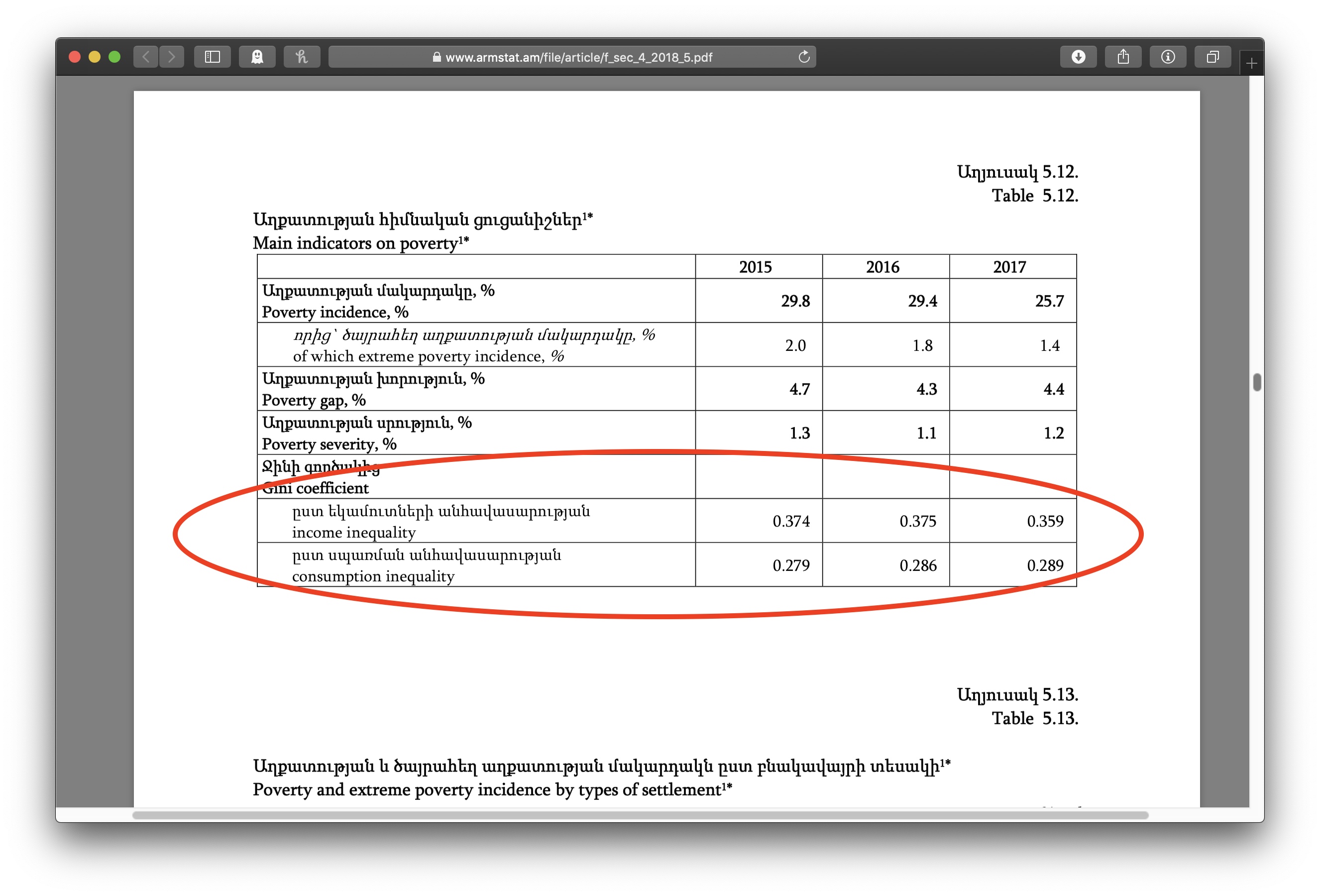
It’s also pretty common to want to get a bunch of files linked from a website. Consider this example from my own work on the Standardized World Income Inequality Database. The SWIID depends on source data on income inequality from international organizations and national statistical offices around the world, including Armenia’s Statistical Committee (ArmStat). ArmStat has a annual report on food security and poverty that includes a chapter titled “Accessibility of Food” that has some data on income and consumption inequality that I want.
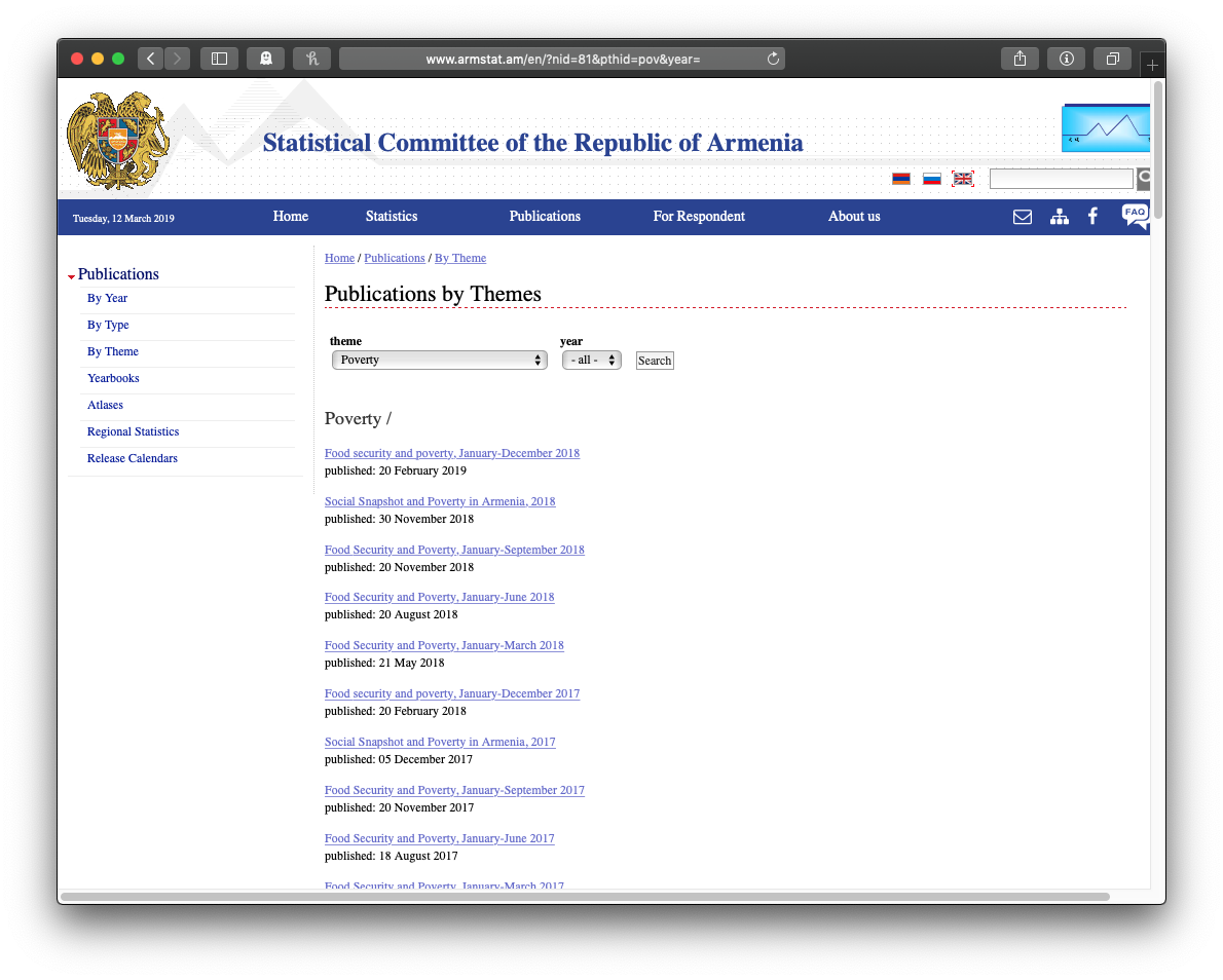
Here’s the page with the list of poverty reports:
Clicking on the top link shows a list of chapters. Note the chapter on “Accessibility of Food”:
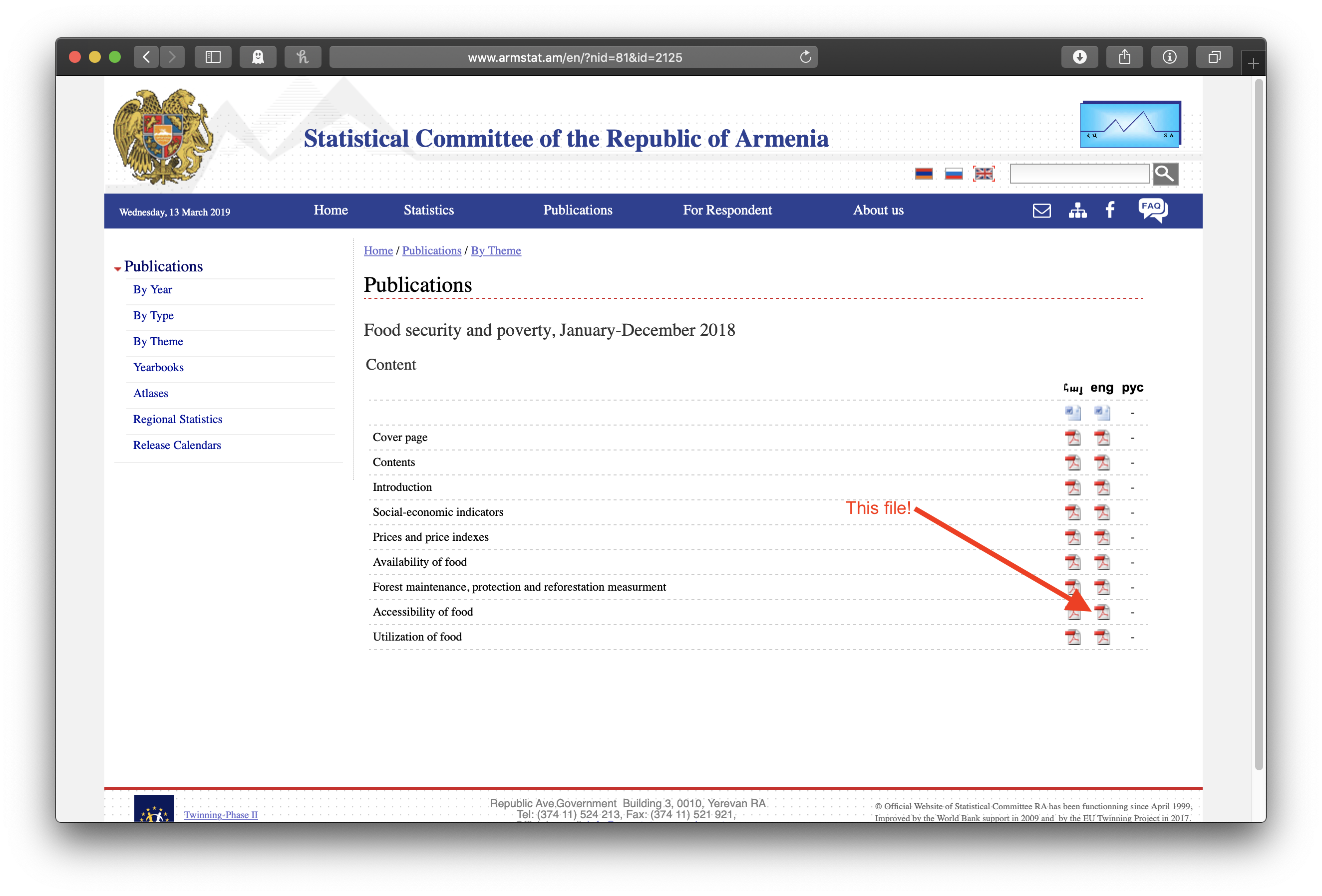
Clicking on that pdf icon shows the pdf file of the chapter, where we can see, if we scroll down a bit, the table with the lovely data:
But again, we want to download that file for that chapter for every one of the annual reports listed on that first page. We could go carefully down the list of all the reports, pick out the annual reports, click through the chapters over and over, but there’s more than a dozen annual reports here, and we’re still at the start of the alphabet as far as countries go. Further, there’ll be another new annual report next year. We need to have this process automated.
Thinking about it a moment, this is maybe a particularly tricky scraping job because we need to:
use rvest to get the links for the reports we want from the main page on poverty, and then
follow each of those links to get the link for the chapter we want, and, after we have all those links, then
we can download all the chapter files and extract the data we want from them. (Reading pdfs into R is another great data acquisition skill, but I think it merits a post of its own, so for now we’ll stop once we have all the files we want.)
In a more straightforward scraping job, step 2 wouldn’t be necessary at all, but this sort of arrangement isn’t all that uncommon (think of articles in issues of journals, for another example), and it will give us a chance to practice some of our data wrangling skills.
And in the very most straightforward cases, as Raman Singh Chhína reminded me here, the links to files we want will fit some consistent pattern, and even step 1 won’t be necessary as we can simply construct the list of links we need along the lines of: needed_links <- str_c("https://suchandsuch.org/files/annualreport", 2006:2018, ".pdf"). Then we can skip straight to step 3.
But let’s roll up our sleeves and take on this harder job.
Step 1: Getting the Links to the Reports
Like with scraping web tables, we will start by pasting our link into read_html(), but now we will need some more information about just which part of the page we want to scrape, information we’ll get from a neat little tool called SelectorGadget. The rvest package includes a nice vignette on how to install and use it here. With SelectorGadget installed in our bookmarks bar (called the favorites bar in Safari here) and engaged (just click on it), each element of the page gets boxed in color as you mouse over it:
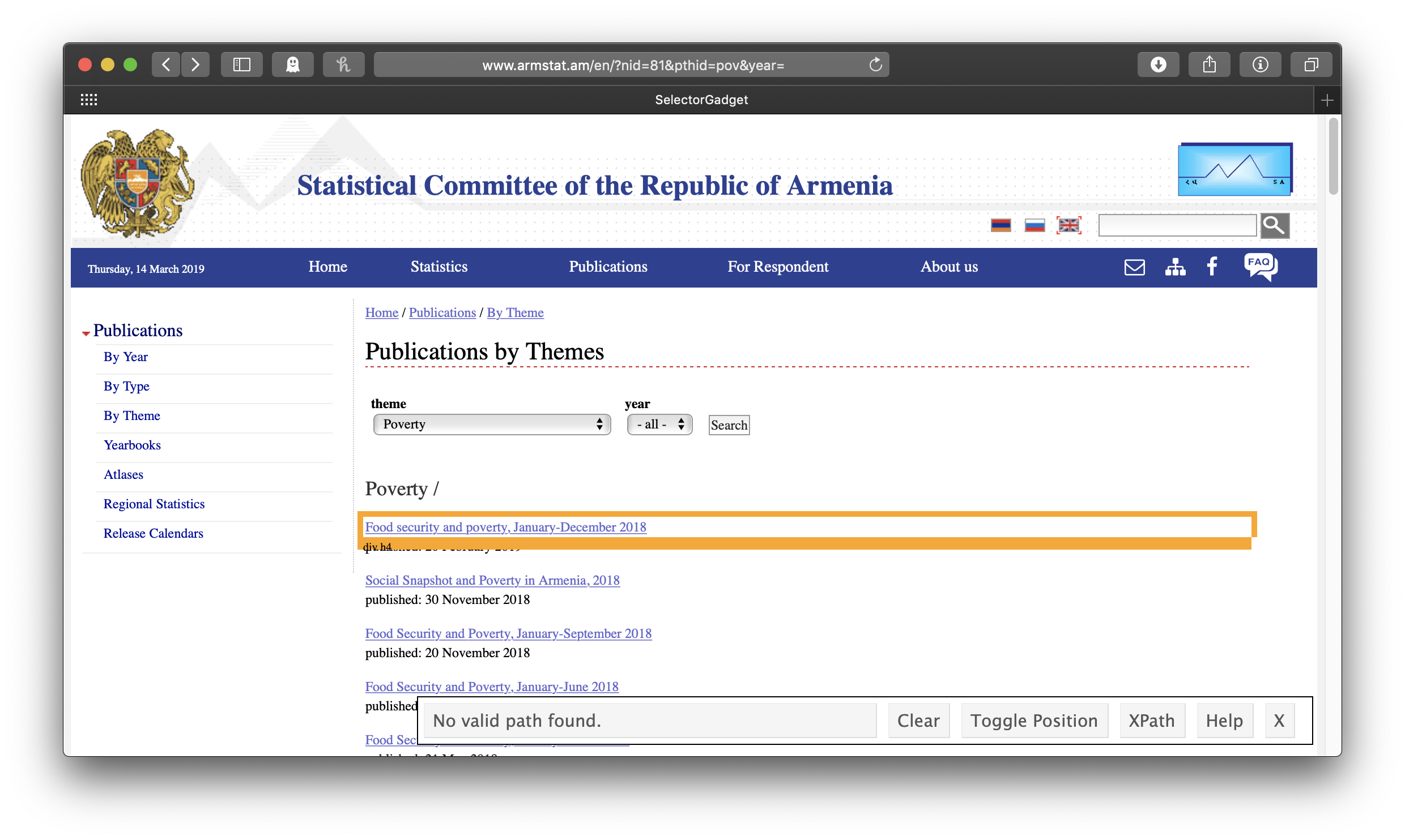
The idea is to get everything you want—and nothing you don’t want—highlighted in green or yellow. Clicking on the first link gives us all the links of the reports . . . but also all the other links:
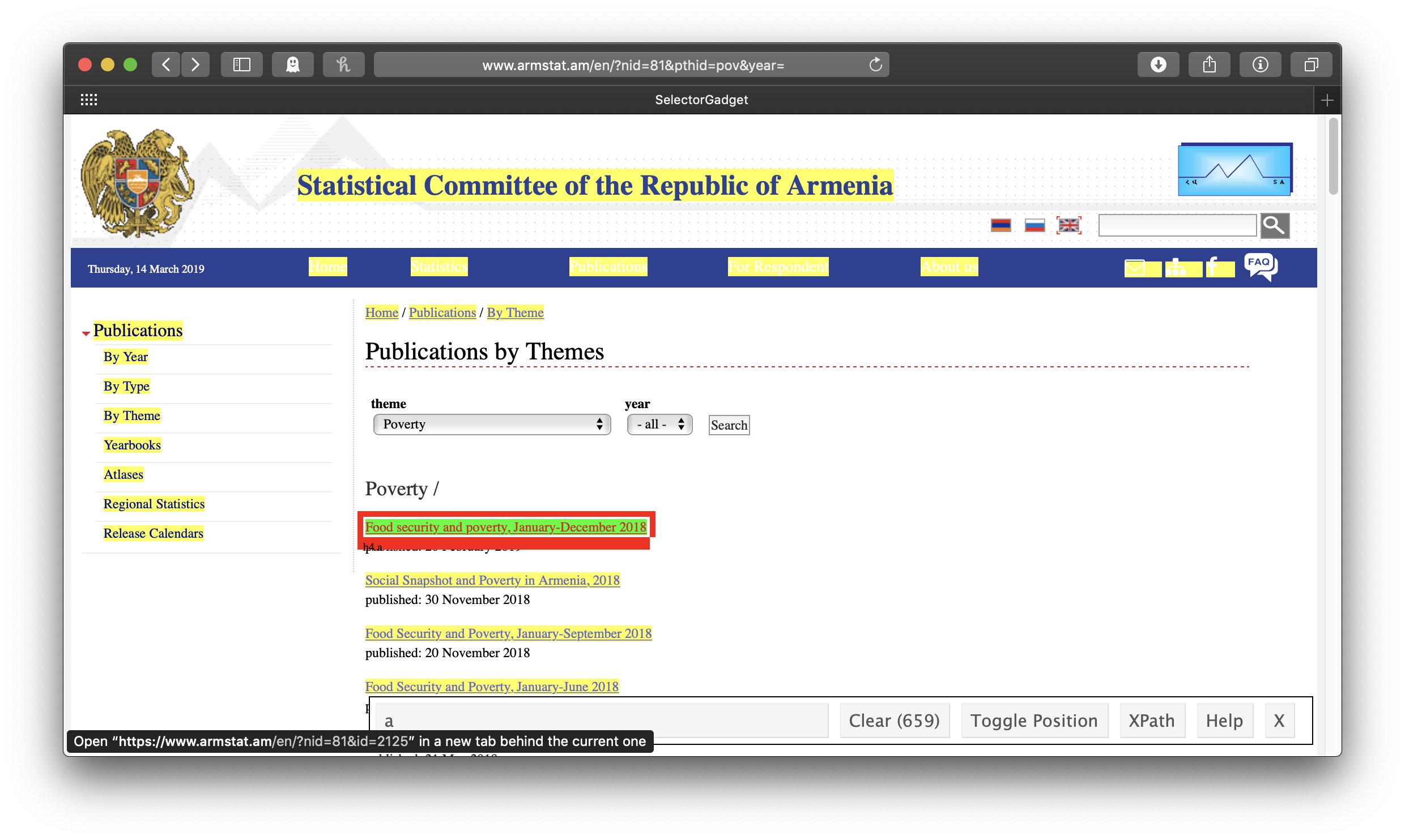
So we click on one of the links we don’t want to turn it red. In this case, this actually leaves us with exactly what we want, just the links of the reports:
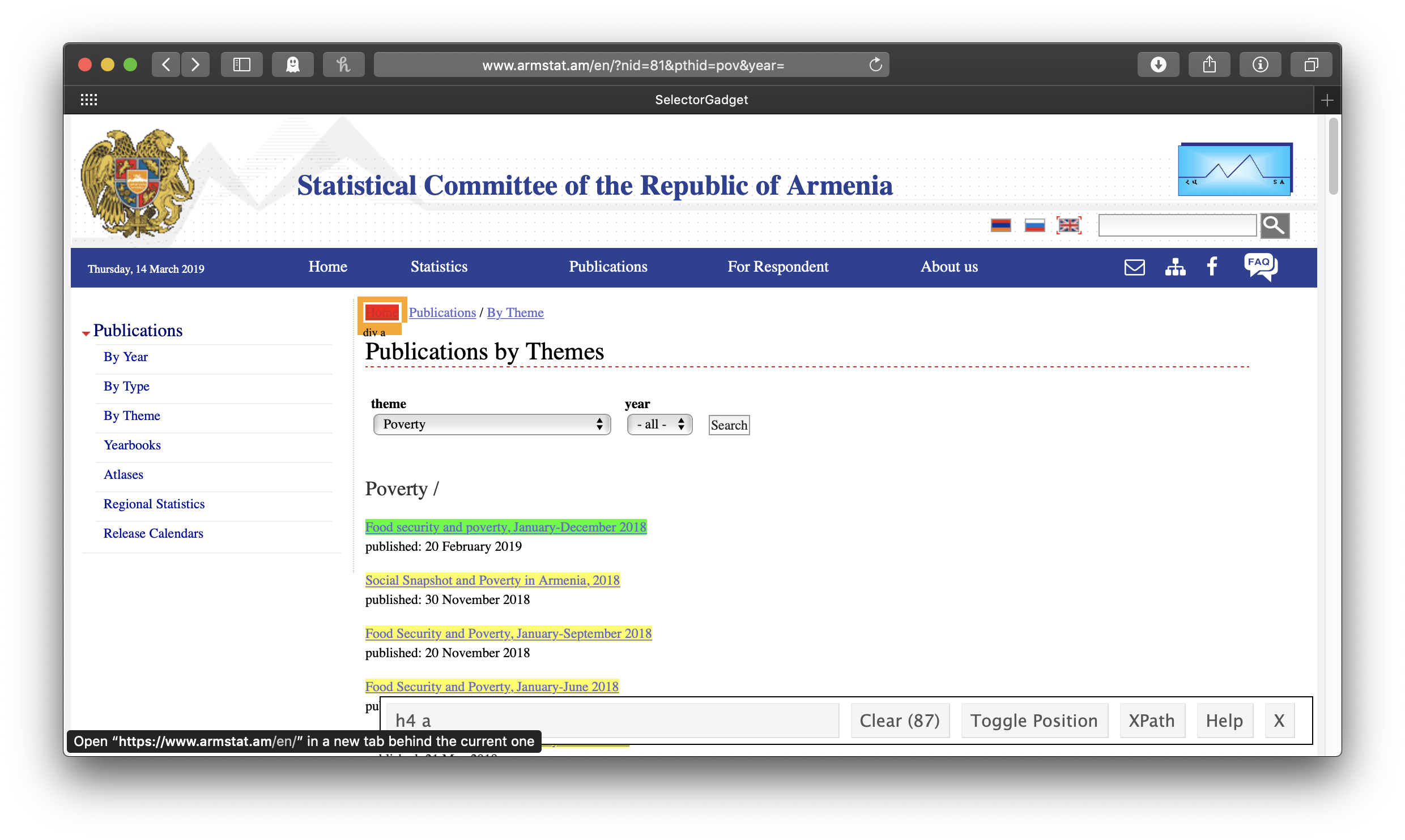
Note that in the wide SelectorGadget box at the bottom of the window, it says “h4 a”—that’s the info we’ll use to identify the parts of the webpage we want, using rvest’s html_nodes() function. This will result in a list of xml nodes. We’ll make a tibble of these nodes, with one variable for the title of the report and one for its link. The report title is just the link text, which we get by passing the node to html_text(); for consistency’s sake (some of the titles of the early reports are in all caps), we’ll make all of the titles lowercase with str_to_lower(). To get the report link url, we use html_attr("href"). In this case, the urls are expressed relative to the ArmStat homepage, so we also need to swap out the dot which stands for that address with the actual address. We only want the year-end reports, so we’ll use the combination of filter() and str_detect() to keep only those that include “december” in their title, and the titles of some reports indicate that they are only available in Armenian, so we’ll filter those out, too.
reports_nodes <- read_html("http://www.armstat.am/en/?nid=81&pthid=pov&year=") %>%
  html_nodes("h4 a")

reports_links <- tibble(report_title = reports_nodes %>%
                                html_text() %>%
                                str_to_lower(),
                            report_link = reports_nodes %>%
                                html_attr("href") %>%
                                str_replace("\\.",
                                            "https://www.armstat.am/en")) %>%
    filter(str_detect(report_title, "december") &
               !str_detect(report_title, "armenian"))

reports_links
## # A tibble: 14 x 2
## report_title report_link
## <chr> <chr>
## 1 food security and poverty, january-dece… https://www.armstat.am/en/?nid=8…
## 2 food security and poverty, january-dece… https://www.armstat.am/en/?nid=8…
## 3 food security and poverty, january-dece… https://www.armstat.am/en/?nid=8…
## 4 food security and poverty, january-dece… https://www.armstat.am/en/?nid=8…
## 5 food security and poverty, january-dece… https://www.armstat.am/en/?nid=8…
## 6 food security and poverty, january-dece… https://www.armstat.am/en/?nid=8…
## 7 food security and poverty, january-dece… https://www.armstat.am/en/?nid=8…
## 8 food security and poverty, january-dece… https://www.armstat.am/en/?nid=8…
## 9 food security and poverty, january-dece… https://www.armstat.am/en/?nid=8…
## 10 food security and poverty, january-dece… https://www.armstat.am/en/?nid=8…
## 11 food security and poverty, january-dece… https://www.armstat.am/en/?nid=8…
## 12 food security and poverty, january- dec… https://www.armstat.am/en/?nid=8…
## 13 food security and poverty january-december… https://www.armstat.am/en/?nid=8…
## 14 food security and poverty january-december… https://www.armstat.am/en/?nid=8…Step 2: Getting the Links to the Chapter Files
Now that we have the links to all of the reports, we need to get the link to the chapter file we want from each one of them. We’ll start with the first report and then use the tidyverse’s iteration tools, map and walk, to apply our code to all of the reports.
Right, so let’s take on that first report. Back to SelectorGadget! Clicking on the link for the first report, engaging SelectorGadget, and clicking on the chapter title “Accessibility of food” gives us the “td” tag, which defines a cell in an html table. This means that each of our chapter nodes will be a separate cell from this web table, and we’ll have to reconstruct the table structure ourselves. If we knew a bit of html, we could use the “tr” tag, which defines rows, instead, and spare ourselves this fancy footwork, but whenever I want to know anything about html I have to look it up. You may be in the same boat, so let’s just plan on doing the footwork.
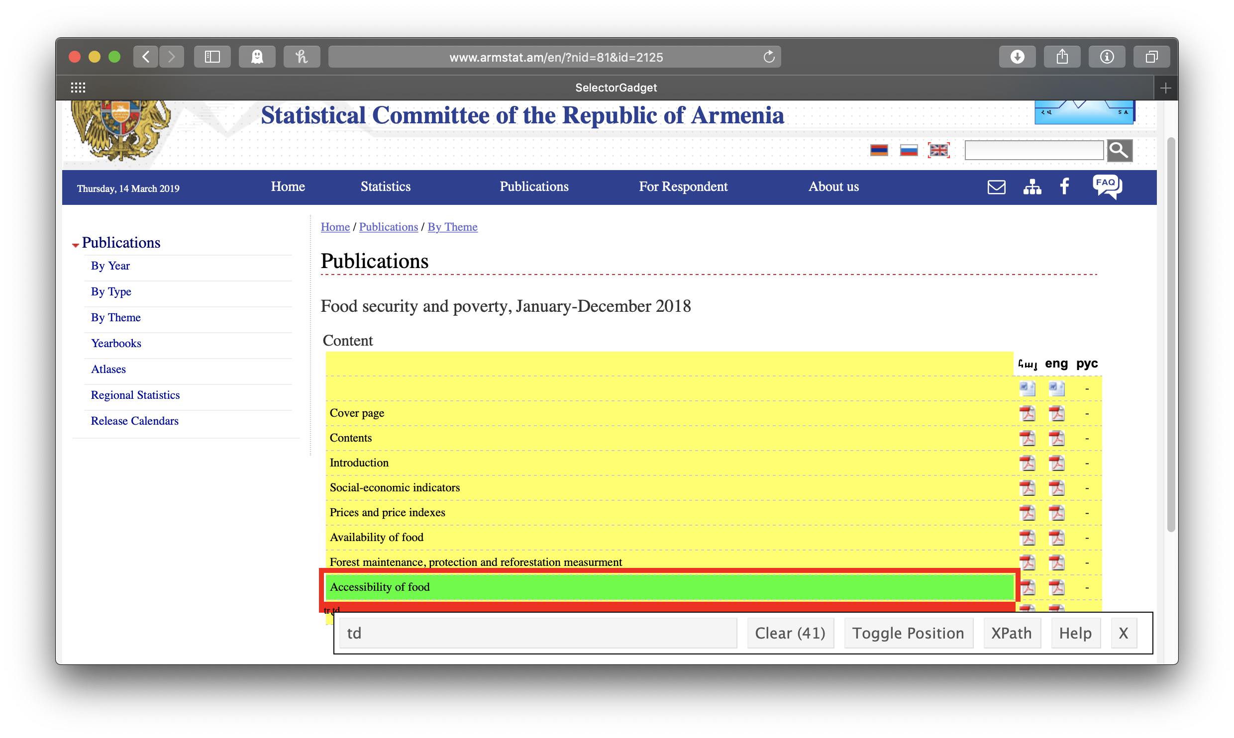
Again, we’ll make a tibble of titles and links from our chapter nodes. Again, we’ll use html_text() to get the titles and standardize on lowercase letters. However, this time, the titles are not themselves links—the links are in subsequent cells in the same row in the table that contain no text at all. We’ll use if_else() to test if the title is an empty string, and if so, set it to NA_character_ (the missing data indicator for strings). We can get the links, meanwhile, by selecting html_node("a")—“a” for anchor defines links in html (we didn’t need to do this separately when we were getting the report links above because our tag, “h4 a”, already included it)—and then html_attr("href") as before. And we’ll have to deal with the relative urls again, too (two dots to replace this time, and no /en—we figure this out by clicking the link in the actual webpage and comparing it to what html_attr("href") gave us). How do we deal with the fact the rows of our tibble are just cells from the webtable, so our titles have no links and our links have no titles? Here comes that “fancy footwork”: we’ll use the fill() function to replace any NAs in our chapter titles with the last observed chapter title (this is why we set the empty strings to NA_character_ the way we did above; fill() only works on NAs, not empty strings). Then, since each link is actually repeated twice—ArmStat understandably wants to be sure you know that their bilingual documents are available to you in both Armenian and English—we use distinct() to get rid of the duplicates. Finally, we drop the observations without links (that is, the original title cells), leaving us with a neat reconstruction of the table of chapter titles and links:
report_link <- reports_links %>%
    pull(report_link) %>%
    first()

chapter_nodes <- read_html(report_link) %>%
    html_nodes("td")

chapter_links <- tibble(chapter_title = chapter_nodes %>%
                            html_text() %>%
                            str_to_lower() %>%
                            if_else(. == "", NA_character_, .),
                        chapter_link = chapter_nodes %>%
                            html_node("a") %>%
                            html_attr("href") %>%
                            str_replace("\\.\\.",
                                        "https://www.armstat.am")) %>%
    fill(chapter_title) %>%
    distinct() %>%
    filter(!is.na(chapter_link))

chapter_links
## # A tibble: 10 x 2
## chapter_title chapter_link
## <chr> <chr>
## 1 " " https://www.armstat.am/file/articl…
## 2 cover page https://www.armstat.am/file/articl…
## 3 contents https://www.armstat.am/file/articl…
## 4 introduction https://www.armstat.am/file/articl…
## 5 "social-economic indicators " https://www.armstat.am/file/articl…
## 6 prices and price indexes https://www.armstat.am/file/articl…
## 7 availability of food https://www.armstat.am/file/articl…
## 8 "forest maintenance, protection and refo… https://www.armstat.am/file/articl…
## 9 accessibility of food https://www.armstat.am/file/articl…
## 10 utilization of food https://www.armstat.am/file/articl…Of course, we just want the “accessibility of food” chapter, and, in fact, really just the link rather than a tibble:
accessibilty_chapter <- chapter_links %>%
    filter(str_detect(chapter_title, "accessibility"))

accessibilty_chapter
## # A tibble: 1 x 2
## chapter_title chapter_link
## <chr> <chr>
## 1 accessibility of food https://www.armstat.am/file/article/f_sec_4_2019_5.pdfjust_the_link <- accessibilty_chapter %>%
pull(chapter_link)
just_the_link## [1] "https://www.armstat.am/file/article/f_sec_4_2019_5.pdf"All right, so now we’re going to take everything we just did to get the link for the first report’s accessibility chapter and wrap it into a function that takes a report link and returns just_the_link for the accessibilty chapter:
get_chapter_link <- function(report_link) {
    chapter_nodes <- read_html(report_link) %>%
        html_nodes("td")

    chapter_links <- tibble(chapter_title = chapter_nodes %>%
                               html_text() %>%
                               str_to_lower() %>%
                               if_else(. == "", NA_character_, .),
                           chapter_link = chapter_nodes %>%
                               html_node("a") %>%
                               html_attr("href") %>%
                               str_replace("\\.\\.", "https://www.armstat.am")) %>%
        fill(chapter_title) %>%
        distinct() %>%
        filter(!is.na(chapter_link))

    accessibilty_chapter <- chapter_links %>%
        filter(str_detect(chapter_title, "accessibility"))

    just_the_link <- accessibilty_chapter %>%
        pull(chapter_link)

    return(just_the_link)
}
Now we can use that function to create a new chapter link variable in our reports_links tibble, with the wrinkle that mutate() expects a vectorized function—that is, one that operates on all the values of the variable at the same time—and, thanks to Jim Hester, we know we can meet this expectation by using map_chr():
reports_links <- reports_links %>%
    mutate(chapter_link = map_chr(report_link, get_chapter_link))

reports_links
## # A tibble: 14 x 3
## report_title report_link chapter_link
## <chr> <chr> <chr>
## 1 food security and pove… https://www.armstat.… https://www.armstat.am/file…
## 2 food security and pove… https://www.armstat.… https://www.armstat.am/file…
## 3 food security and pove… https://www.armstat.… https://www.armstat.am/file…
## 4 food security and pove… https://www.armstat.… https://www.armstat.am/file…
## 5 food security and pove… https://www.armstat.… https://www.armstat.am/file…
## 6 food security and pove… https://www.armstat.… https://www.armstat.am/file…
## 7 food security and pove… https://www.armstat.… https://www.armstat.am/file…
## 8 food security and pove… https://www.armstat.… https://www.armstat.am/file…
## 9 food security and pove… https://www.armstat.… https://www.armstat.am/file…
## 10 food security and pove… https://www.armstat.… https://www.armstat.am/file…
## 11 food security and pove… https://www.armstat.… https://www.armstat.am/file…
## 12 food security and pove… https://www.armstat.… https://www.armstat.am/file…
## 13 food security and poverty… https://www.armstat.… https://www.armstat.am/file…
## 14 food security and poverty… https://www.armstat.… https://www.armstat.am/file…Step 3: Getting! All! the! Files!
This is actually straightforward, now that we have a tibble of report titles and links to chapter files. The download.file() function will save the contents of a link (its first argument) to a filepath (its second argument) and the walk2() function allows you to pass a pair of vectors to a function to iteratively use as its two arguments (first the first element of each vector, then the second element of each vector, and so on). We’ll use str_extract() to get the year of the report from its title, and use it to make a file name for the pdf with str_c(). But first we should create a directory to save those files in. And after each download, we’ll insert a brief pause with Sys.sleep(3) to be sure that were not hammering the server too hard. Maybe not really necessary this time, given that we’re getting just 14 files, but it’s the considerate thing to do and a good habit.
dir.create("armstat_files")

walk2(reports_links$report_title, reports_links$chapter_link,
      function(report_title, chapter_link) {
    pdf_path <- file.path("armstat_files",
                          str_c("armstat",
                                str_extract(report_title, "\\d{4}"),
                                ".pdf"))
    download.file(chapter_link, pdf_path)
    Sys.sleep(3)
})
And that’s that. And remember, use your new powers for good, not for evil. Be sure to respect the terms of service of any website you might want to scrape.
Remember, if you haven’t installed it before, you will need to download
janitorto your machine withinstall.packages("janitor")before this code will work.↩︎